Background
For the past two summers, I have interned at the GMU Center for Intelligent Spatial Computing, where a number of PhD students are working on very interesting computational geoinformatics projects. One of the projects which I contributed to was the NASA Goddard/NSF Planetary Defense Project - an endeavor focused on the mitigation of asteroid threats to our planet through means of developing a large knowledge base of information about NEOs (Near Earth Objects), which can be accessed by scientists and engineers throughout the world.
The Tedious Problem
In order to gather relevant information to store in this knowledge base, a webcrawler was implemented using Apache Nutch with customized source code. After a set of seed URL’s was configured, the webcrawler returned 30,000+ websites in a single crawl session, all of which were ideally related to the Planetary Defense project.
How could the effectiveness of this webcrawler be tested? In other words, how could we know how many websites which were crawled were actually relevant to the Planetary Defense Project?
The most straightforward method was of course manual evaluation of the webpages, i.e. a human or group of humans going through all 30,000 webpages to label whether a certain webpage was relevant or not for all webpages. As expected, this proved to be a pain in the ass, time consuming task for a group of relatively smart people who no longer live in the stone age.
The solution? A buzzword known as “machine learning,” of course.
Building a Text Classifier in Python
The first approach to solve this problem was building a text classifier in the Python language. Instead of manually going through the webcrawling results each time using human evaluation, the text classifier would be fed the results of the crawl in the form of a parsed URL and title for each result, and then predict whether or not the website was relevant. Of course, the text classifier would have to be fed a training set of data to be, well, trained.
In other words, it was necessary that a human or group of humans manually evaluate an entire crawl session result to train the classifier, and this is exactly what we did. After agreeing upon a certain criteria of relevancy for each website, another intern and I went over all ~30,000 pages ourselves and marked them as relevant, not relevant, or maybe relevant.
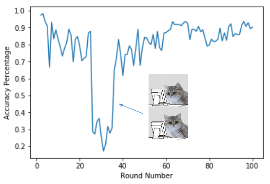
The above image is a calculated accuracy percentage for each round after going through the webpages manually. You can probably guess where, but there was an unexpected and extreme dip in accuracy relatively early on in the crawl.
Creating Training Data
Originally, the crawling results were in a CSV file. We wanted to extract two things from each website: a parsed URL without any special characters like “/” etc., and a parsed title, again, without any special characters like commas or periods. The parsed results for each and every website from the CSV file were then stored in a corresponding text file which would later be opened up by the text classifier.
import csv
import re

"""
Creates dataset of text documents containing only words inside of pasred URL and title for each
crawl result.
"MAYBE" no longer needed and can be deleted.
NOTE: User of program must edit paths accordingly
"""

# put csv file into list
with open(r'C:\JGSTCWork\Crawler Classification\balancedSet.csv', encoding="utf8") as csv_file:
    reader = csv.reader(csv_file, delimiter = ",")
    data = list(reader)

for row in range(0, len(data)):

    parsedURL = re.findall(r"['\w']+", data[row][0])
    parsedTitle = re.findall(r"['\w']+", data[row][1])

    if data[row][6] == 'Maybe':
        with open('C:\\JGSTCWork\\Crawler Classification\\WebpageData\\MAYBE\\' + 'MAYBE' + str(row) + '.txt', 'w', encoding="utf8") as title:
            urlString = ''
            for i in range(0, len(parsedURL)):
                if parsedURL[i] != 'http' and parsedURL[i] != 'https' and parsedURL[i] != 'www':
                    urlString = urlString + ' ' + parsedURL[i]
            title.write(urlString)

            titleString = ''
            for i in range(0, len(parsedTitle)):
                titleString = titleString + ' ' + parsedTitle[i]
            title.write(titleString)
    if data[row][6] == 'Yes':
        with open('C:\\JGSTCWork\\Crawler Classification\\WebpageData\\YES\\' + 'YES' + str(row) + '.txt', 'w', encoding="utf8") as title:
            urlString = ''
            for i in range(0, len(parsedURL)):
                if parsedURL[i] != 'http' and parsedURL[i] != 'https' and parsedURL[i] != 'www':
                    urlString = urlString + ' ' + parsedURL[i]
            title.write(urlString)

            titleString = ''
            for i in range(0, len(parsedTitle)):
                titleString = titleString + ' ' + parsedTitle[i]
            title.write(titleString)
    if data[row][6] == 'No':
        with open('C:\\JGSTCWork\\Crawler Classification\\WebpageData\\NO\\' + 'NO' + str(row) + '.txt', 'w', encoding="utf8") as title:
            urlString = ''
            for i in range(0, len(parsedURL)):
                if parsedURL[i] != 'http' and parsedURL[i] != 'https' and parsedURL[i] != 'www':
                    urlString = urlString + ' ' + parsedURL[i]
            title.write(urlString)

            titleString = ''
            for i in range(0, len(parsedTitle)):
                titleString = titleString + ' ' + parsedTitle[i]
title.write(titleString)
As you can see, I first created a regular expression to extract the alphanumeric characters only for each website URL and title. Afterwards, I noted that words like “www” should not be included for each result, as they would not contribute to improved results since they were shared by each result. The parsed and formatted URL and title for each website was stored in a string which would be fed into the text classifier. It’s certainly not the prettiest Python script I’ve written, but it got the job done.
Naive Bayes Classifier
After the training set was created, I made a multinomial Naive Bayes classifier using scikit-learn. This was quite a long Python script, so I will not insert the entire code block here.
Essentially, the script utilized both a count vectorizer and a classifier to divide a website into a relevant or not relevant category. The count vectorizer used 3-grams. These two methods were then fit on the training data.
pipeline = Pipeline([
    ('count_vectorizer',   CountVectorizer(ngram_range=(1,  3))), # looking for n-gram frequency
    ('classifier', MultinomialNB())])

pipeline.fit(data['text'].values, data['class'].values)
After using 6-fold cross validation, we ended up with an F1 Score of .84 for the “relevant” class.
Here is the full Python script.
Elastic Net Models in R
I like variety in what I do, so I figured that I would create a text classification model in a language that I am much more experienced in and benchmark the results of this. Afterall, we are trying to find the model which provides us with the most accurate results.
Creating the Training, Testing, and Validation Labels
I used the following libraries for this code.
library(readr)
library(dplyr)
library(ggplot2)
library(methods)
library(stringi)
library(smodels)
library(tokenizers)
The first thing that I did was import the data, and much like in my Python script, I extracted the alphanumeric characters from the URL and title by using a regular expression. The validation, training, and testing labels were then assigned to each row of my dataset.
pd$url <- stri_replace_all(pd$V1, " ", regex = "[^A-Za-z]+")
pd$title <- stri_replace_all(pd$V2, " ", regex = "[^A-Za-z]+")
pd$text <- paste(pd$url, pd$title, sep=" ") #combine URL and title
pd$relevant <- pd$V7
pd <- pd[,c(10, 11)]

pd$relevant <- as.factor(pd$relevant)
pd$relevant <- as.integer(pd$relevant)

#add train, text, valid
coff <- runif(nrow(pd))
pd$train_id <- "valid"
pd$train_id[coff < .6] <- "train"
pd$train_id[coff > .8] <- "test"
Basic Elastic Net
The first step of building the model was creating the dataframe containing the features of the text for each website.
token_list <- tokenize_words(pd$text)
token_df <- term_list_to_df(token_list)
X <- term_df_to_matrix(token_df, min_df = 0.01, max_df = 0.90,
                       scale = TRUE)

y <- pd$relevant
X_train <- X[pd$train_id == "train",]
X_valid <- X[pd$train_id == "valid",]
y_train <- y[pd$train_id == "train"]
y_valid <- y[pd$train_id == "valid"]
I then built a basic elastic net model, taking note of what the most important keywords were for each category: maybe relevant, not relevant, and relevant.
This is quite interesting. For example, it appears that the word “human” is highly positively correlated with a webpage not being relevant. On the other hand, “bodies” and “comets” are positively correlated with a webpage being relevant. These are all to be expected, and this is a good sign.
(Intercept)    -1.7036060  7.655788e-01  9.380273e-01
www             .          1.275738e+00  .
space           .          3.501563e-01  .
nasa            1.1106041  .             .
spaceref        2.5091489  .             .
html            .          .             6.558025e-01
com             .          4.308986e-01  .
https           .          .             3.462334e-01
int             .          .             7.156397e+00
images          .          3.871393e-03  .
in              .          3.183568e+00  .
our             .         -1.519176e+00  1.693031e+00
spaceflight     .          1.599540e+00  .
human           .          8.603843e+00  .
and            -0.5390742  .             .
blog            .          .             2.075478e-01
org             1.6390389  .             .
for             .          .            -1.474122e+00
edu             .         -1.372681e+00  .
gemini          .         -1.468051e-01  .
on              .          .             3.283170e-01
to              .          .            -1.765228e+00
s               .          .             9.162627e-01
spaceinimages   .          2.122917e+01  .
a               .          6.817651e-01  .
pdf             .          .            -2.310649e+00
nss            -0.9275909  1.314012e+00  .
exploration     .         -1.491643e+00  .
mission         .         -5.686946e+00  .
solar           .         -6.480667e+00  .
science         5.1060115  .             .
rosetta         .         -1.101810e+00  3.193344e+00
mars            .          .             3.649263e+00
m               0.8589970 -3.926608e+00  .
from            .          4.621237e+00 -1.833344e+00
tag             .          .             8.789845e-01
at              .          7.765477e-01  .
tl              .          1.191679e+01  .
society         .          .             6.256270e+00
sservi          .          1.649096e+00  .
feed            .          7.371971e+00  .
atv             .         -4.422721e+00  .
main            .          8.501298e+00  .
international   5.1961228  .             .
de              .          7.304046e-01  .
index           .         -3.663839e+00  .
station         .          .             6.704107e+00
multimedia      .         -1.219405e+00  .
videos          .          .            -1.174784e+00
comet           .          .             1.720822e+01
earth           .          6.938648e+00  .
moon            .         -5.106245e+00  1.484604e+00
hack            8.9953919  .             .
launch          .         -1.291164e+00  .
gallery         .          3.648870e+00 -4.809539e+00
null            .          7.119583e-01 -6.969904e-01
asp             .          2.138041e+00  .
first           .          .            -6.364356e-01
is              .          3.745857e+00  .
htv             .          .             6.424223e-01
new             0.8737653 -1.464462e+00  .
ca              .          2.355993e+00  .
onorbit         .          .            -3.254936e-01
jp              .          2.408248e+00 -2.896212e+00
blogs           .          .             5.791957e+00
jpl             .          2.315183e+00  .
agency          .          2.670649e+00  .
lunar           .         -4.456191e+00  .
astronomy       .          1.482613e+00  .
video           .          .            -1.528798e+00
comments        .          .             1.948771e+00
education       .          5.840651e+00  .
image           .          .             1.581746e+00
data            .         -4.060699e+00  5.996692e-01
astronaut       .          1.035901e-02 -6.654837e+00
media           .          1.001119e+00  .
chaser          .          .             4.887039e+00
vehicle         .          .             5.741671e+00
planetary       .          .             2.003738e+01
business        .          3.835389e+00  .
seen            .          3.520356e-01 -4.759763e-01
print           .         -4.686986e+00  .
about           .          .             1.484135e+00
missions        .         -6.440440e-01  .
technology      .          .            -7.238664e-02
day             .          .             5.764199e-01
transfer        .          3.410509e+00  .
u               .          .             2.009586e-01
crew            .          1.245603e+01  .
doc             .          .             7.320697e+00
h               .          1.758862e+00  .
microsoft       .          6.499480e-01  .
word            .          3.816761e-15  .
desktopdefault  .          .             7.157579e-02
tabid           .          .             5.505700e-15
small           .          .             6.465534e+00
view            .          .            -9.883828e-01
it              .          2.924517e-01  .
page            .         -1.438374e+00  1.675854e+00
read            .          .             1.050150e+01
telescope       .         -2.791263e+00  .
exoplanets      .          .             1.269019e+01
flight          .          .            -1.177459e+00
php             .          1.824602e+00 -2.515165e+00
embed           .          4.975975e-01 -3.260299e+00
ro              .          .            -2.311466e-01
kounotori       .          .             1.767315e+01
sciops          .          .             8.339759e+00
programs        .          .             1.365461e+00
web             .         -1.401224e+00  .
bodies          .          .             1.080721e+01
solarviews      .          .             3.217479e+00
Predictions were then made on the dataset, and the testing, training, and validation were calculated, giving a final testing rate of around 64.5% - better than a random guess which would’ve yielded 33%.
pd$relevant_pred <- predict(model, newx = X, type = "class")
tapply(pd$relevant_pred == pd$relevant,
       pd$train_id, mean)
test: 0.6450079
train: 0.6677614
valid: 0.6280193
N-Gram Testing
To improve the accuracy of the text classifier, I experimented with different n-gram tokenizers, finding that trigrams yielded the best result.
token_list <- tokenize_ngrams(pd$text, n_min = 1, n = 3)
token_df <- term_list_to_df(token_list)
X2 <- term_df_to_matrix(token_df, min_df = 0.01, max_df = 0.90,
                       scale = TRUE)
X <- cbind(X, X2)

y <- pd$relevant
X_train <- X[pd$train_id == "train",]
X_valid <- X[pd$train_id == "valid",]
y_train <- y[pd$train_id == "train"]
y_valid <- y[pd$train_id == "valid"]
The inclusion of this method slightly improved training and validation rates, but not testing.
model <- cv.glmnet(X_train, y_train, nfolds = 6, family = "multinomial")
pd$relevant_pred <- predict(model, newx = X, type = "class")
tapply(pd$relevant_pred == pd$relevant,
       pd$train_id, mean)
test: 0.6450079
train: 0.6940339
valid: 0.6392915
To see if I could get even better results, I also included a character shingle model. My model was now being trained on a dataset comprised of basic test data, data containing trigrams, and data containing character shingles.
token_list <- tokenize_character_shingles(pd$text, n_min = 1, n = 3)
token_df <- term_list_to_df(token_list)
X3 <- term_df_to_matrix(token_df, min_df = 0.01, max_df = 0.90,
                       scale = TRUE)
X <- cbind(X, X2, X3)
y <- pd$relevant
X_train <- X[pd$train_id == "train",]
X_valid <- X[pd$train_id == "valid",]
y_train <- y[pd$train_id == "train"]
y_valid <- y[pd$train_id == "valid"]
This led to some overfitting, but improved testing, training, and validation rates.
model <- cv.glmnet(X_train, y_train, nfolds = 7, family = "multinomial")
pd$relevant_pred <- predict(model, newx = X, type = "class")
tapply(pd$relevant_pred == pd$relevant,
       pd$train_id, mean)
test: 0.6862124
train: 0.7542419
valid: 0.6682770
Ultimately, this was the best model. A neural network is currently in the making as well.
Thoughts
The objective was accomplished, and text classification models were developed in Python using a Multinomial Naive Bayes classifier and in R using an Elastic Net. Both yield relatively good results and both help with the task of eliminating the need for human evaluation of webcrawler results.
At this point, it’s simply a matter of tweaking our text classifiers and training data until we get a classification rate we are truly happy with and willing to accept as a standard for evaluating the webpages for the Planetary Defense project.
It is definitely worth noting that the Python training data only included relevant and not relevant webpages, while the training data for the R model included relevant, not relevant, and maybe labels. Interestingly enough, the “maybe” label is where there was the most confusion in the model, and this may come down to human error: what my colleague and I thought was “maybe” relevant can be completely different.
Consequently, the data which the model was trained on is at fault here, and better results can be gotten with the elimination of the “maybe” label or a completely new and unbiased set of training data.